FastScapeLib is an interface or library (i.e. a set of subroutines) to model landscape evolution by river incision, sediment transport and deposition in continental and marine environments.
FastScapeLib is a set of routines that solve (a) the stream power law (SPL) that has been enriched by a sediment transport/deposition term (see Yuan et al, 2019a in References) (b) hillslope diffusion and (c) marine transport and deposition (see Yuan et al, 2019b in References), using a set of highly efficient algorithms that are all \(\mathcal{O}(n)\) complexity and implicit in time. These routines can be called from a Fortran, C or Python main program and are ideally suited to be coupled to a tectonic model, be it very simple, such as a flexural isostatic model, or very complex, such as a 3D thermo-mechanical model.
Basic partial differential equation solved by FastScapeLib is:
where \(h\) is topography, \(U\) is uplift, \(S\) is slope, \(A\) is drainage area, and \(K_f\), \(m\), \(n\), \(G\) and \(K_d\) are parameters (see further down for unit and meaning).
Build and install FastScapeLib
FastScapeLib is not yet available as a binary package, so you need to build and install it manually.
Download the source files
First, download the sources using git:
git clone https://github.com/fastscape-lem/fastscapelib-fortran
Alternatively, you can visit the URL of the source repository (https://github.com/fastscape-lem/fastscapelib-fortran) and download the source files as an archive (see the "clone or download button").
Requirements
To build FastScapelib, you need a Fortran compiler (e.g., gfortran,
part of GCC) and CMake (https://cmake.org/). Both can easily be
installed on major platforms, e.g., using Homebrew on MacOS or apt-get
on Linux/Debian. GCC compilers are also available for Windows platforms
(see http://www.mingw.org/).
Build using CMake
Run the following commands from the source directory to build the FastScapeLib Fortran library:
mkdir build
cd build
cmake <options> ..
make
There are several build options, here shown with their default values:
-
-DBUILD_FASTSCAPELIB_STATIC=ON: build fastscapelib as a static library -
-DBUILD_FASTSCAPELIB_SHARED=OFF: build fastscapelib as a shared library -
-DUSE_FLEXURE=OFF: include flexure routines in the library -
-DBUILD_EXAMPLES=OFF: "build usage examples that are in the 'examples' directory
Install the Fortran library
If you want to install the FastScapeLib Fortran static/shared libraries in your system, then simply run:
make install
You should now be able to link your programs using FastScapeLib
routines, e.g., with -lfastscapelib_fortran. See some Fortran programs
in the 'examples' folder.
Install the Python package (using conda)
|
If you want to use this tool from within Python, you may consider using the FastScape package instead, which is built on top of FastScapeLib and which provides a high-level, user-friendly interface. See https://fastscape.readthedocs.io. |
FastScapeLib's Python bindings are available as a conda package (https://docs.conda.io/en/latest/). Conda can be installed from https://docs.conda.io/en/latest/miniconda.html.
Then run the following command:
conda install fastscapelib-f2py -c conda-forge
You should now be able to import the package from within Python, e.g.,
>>> import fastscapelib_fortran as fs
There is a Jupyter notebook in the 'examples' folder showing simple usage of the library.
Install the Python package (from source)
You can also install FastScapeLib's Python bindings from source, e.g, for
development purpose. Run the following command from the source directory (i.e.,
the top-level folder containing the file setup.py):
python -m pip install .
This will also temporarily install all the tools needed to build the package (except a Fortran compiler, which must be already installed). Note: you need pip >= 10.
If you experience issues when installing or importing the package (NumPy compatibility issues), try running pip without build isolation:
python -m pip install . --no-build-isolation
Note that in this case you may first need to manually install all the tools required to build the package (i.e., CMake, NumPy, scikit-build).
Fortran API
FastScapeLib contains the following routines:
FastScape_Init
This routine must be called first, i.e. before calling any other subroutine of the inteface. It resets internal variables.
This routine has no argument:
FastScape_Init ()
FastScape_Set_NX_NY
This routine is used to set the resolution of the landscape evolution model. It must be called immediately after FastScape_Init.
Arguments:
FastScape_Set_NX_NY ( nx, ny)
nx-
Resolution or number of grid points in the x-direction (integer)
ny-
Resolution or number of grid points in the y-direction (integer)
|
|
FastScape_Setup
This routine creates internal arrays by allocating memory. It must be called right after FastScape_Set_NX_NY.
This routine has no argument:
FastScape_Setup ()
FastScape_Set_XL_YL
This routine is used to set the dimensions of the model, xl and yl in meters
Arguments:
FastScape_Set_XL_YL ( xl, yl)
xl-
x-dimension of the model in meters (double precision)
yl-
y-dimension of the model in meters (double precision)
FastScape_Set_DT
This routine is used to set the time step in years
Arguments:
FastScape_Set_DT (dt)
dt-
length of the time step in years (double precision)
FastScape_Init_H
This routine is used to initialize the topography in meters
Arguments:
FastScape_Init_H ( h)
h-
array of dimension
(nx*ny)containing the initial topography in meters (double precision)
FastScape_Init_F
This routine is used to initialize the silt fraction
Arguments:
FastScape_Init_F( F)
F-
array of dimension
(nx*ny)containing the initial silt fraction (double precision)
FastScape_Set_Erosional_Parameters
This routine is used to set the continental erosional parameters
Arguments:
FastScape_Set_Erosional_Parameters ( kf, kfsed, m, n, kd, kdsed, g, gsed, p)
kf-
array of dimension
(nx*ny)containing the bedrock river incision (SPL) rate parameter (or Kf) in meters (to the power 1-2m) per year (double precision) kfsed-
sediment river incision (SPL) rate parameter (or Kf) in meters (to the power 1-2m) per year (double precision); note that when
kfsed < 0, its value is not used, i.e., kf for sediment and bedrock have the same value, regardless of sediment thickness
|
bedrock refers to situations/locations where deposited sediment thickness is less than 1 meter, whereas sediment refers to situations/locations where sediment thickness is greater than 1 meter |
m-
drainage area exponent in the SPL (double precision)
n-
slope exponent in the SPL (double precision)
|
Valuers of |
kd-
array of dimension
(nx*ny)containing the bedrock transport coefficient (or diffusivity) for hillslope processes in meter squared per year (double precision) kdsed-
sediment transport coefficient (or diffusivity) for hillslope processes in meter squared per year (double precision; )note that when
kdsed < 0, its value is not used, i.e., kd for sediment and bedrock have the same value, regardless of sediment thickness g-
bedrock dimensionless deposition/transport coefficient for the enriched SPL (double precision)
|
When |
gsed-
sediment dimensionless deposition/transport coefficient for the enriched SPL (double precision); note that when
gsed < 0, its value is not used, i.e., g for sediment and bedrock have the same value, regardless of sediment thickness p-
slope exponent for multi-direction flow; the distribution of flow among potential receivers (defined as the neighbouring nodes that define a negative slope)is proportional to local slope to power
p
|
|
|
|
FastScape_Set_Marine_Parameters
This routine is used to set the marine transport/compaction parameters
Arguments:
FastScape_Set_Marine_Parameters ( SL, p1, p2, z1, z2, r, L, kds1, kds2)
SL-
sea level in meters (double precision)
p1-
reference/surface porosity for silt (double precision)
p2-
reference/surface porosity for sand (double precision)
z1-
e-folding depth for exponential porosity law for silt (double precision)
z2-
e-folding depth for exponential porosity law for sand (double precision)
r-
silt fraction for material leaving the continent (double precision)
L-
averaging depth/thickness needed to solve the silt-sand equation in meters (double precision)
kds1-
marine transport coefficient (diffusivity) for silt in meters squared per year (double precision)
kds2-
marine transport coefficient (diffusivity) for sand in meters squared per year (double precision)
|
When |
FastScape_Set_BC
This routine is used to set the boundary conditions
Arguments:
FastScape_Set_BC ( ibc)
ibc-
ibcis made of four digits which can be one or zero (ex:1111or0101or1000); each digit corresponds to a type of boundary conditions (0= reflective and1= fixed height boundary); when two reflective boundaris face each other they become cyclic. The four bonudaries of the domain correspond to each of the four digits of ibc; the first one is the bottom boundary (y=0), the second is the right-hand side boundary (x=xl), the third one is the top boundary (y=yl) and the fourth one is the left-hand side boundary (x=0) (integer).

ibc.|
The fixed boundary condition does not imply that the boundary cannot be uplifted; i.e. the uplift array can be finite (not nil) on fixed height boundaries. To keep a boundary at base level, this must be specified in the uplift rate array, |
FastScape_Set_U
This routine is used to set the uplift velocity in meters per year
Arguments:
FastScape_Set_U ( u)
u-
array of dimension
(nx*ny)containing the uplift rate in meters per year (double precision)
|
A fixed boundary condition does not imply that the boundary cannot be uplifted; i.e. the uplift array can be finite (not nil) on fixed height boundaries. To keep a boundary at base level, this must be specified in the uplift rate array, |
FastScape_Set_V
This routine is used to set the advection horizontal velocities in meters per year
Arguments:
FastScape_Set_V ( ux, uy)
ux-
array of dimension
(nx*ny)containing the advection x-velocity in meters per year (double precision) uy-
array of dimension
(nx*ny)containing the advection y-velocity in meters per year (double precision)
FastScape_Set_Precip
This routine is used to set the precipitation rate in meters per year
Arguments:
FastScape_Set_Precip ( p)
p-
array of dimension
(nx*ny)containing the relative precipitation rate, i.e. with respect to a mean value already contained inKfandg(double precision)
|
The value of this array should be considered as describing the spatial and temporal variation of relative precipitation rate, not its absolute value which is already contained in the definition of |
FastScape_Execute_Step
This routine is used to execute one time step of the model
This routine has no argument:
FastScape_Execute_Step ()
FastScape_Get_Step
This routine is used to extract from the model the current time step
Arguments:
FastScape_Get_Step ( istep)
istep-
step number; this counter is incremented by one unit each time the routine
FastScape_Execute_Stepis called; its initial value is 0 (integer)
FastScape_Set_H
This routine is used to set the topography in meters
|
This routine can be used to artificially impose a value to |
Arguments:
FastScape_Set_H ( h)
h-
array of dimension
(nx*ny)containing the topography in meters (double precision)
FastScape_Set_Basement
This routine is used to set the basement height in meters
Arguments:
FastScape_Set_Basement ( b)
b-
array of dimension
(nx*ny)containing the basement height in meters (double precision)
FastScape_Set_All_Layers
This routine is used to increment (or uplift) the topography h, the basement height b and the stratigraphic horizons
Arguments:
FastScape_Set_All_Layers ( dh)
dh-
array of dimension
(nx*ny)containing the topographic increment in meters to be added to the topographyh, the basementband the stratigraphic horizons created when the Stratigraphy option has been turned on by calling theFastScape_Stratiroutine (double precision)
FastScape_Set_Tolerance
This routine can be used to set the convergence parameters for the Gauss-Seidel iterations performed while numerically solving the Stream Power law.
Arguments:
FastScape_Set_Tolerance ( tol_relp, tol_absp, nGSStreamPowerLawMaxp)
tol_relp-
relative tolerance (applied to the current max. topographic elevation)
tol_absp-
absolute tolerance
nGSStreamPowerLawMaxp-
maximum number of Gauss-Seidel iterations
FastScape_Get_GSSIterations
This routine is used to get the actual number of Gauss-Seidel iterations performed while numerically solving the Stream Power law during the last time step.
Arguments:
FastScape_Get_GSSIterations ( nGSSp)
nGSSp-
number of Gauss-Seidel iterations
FastScape_Copy_H
This routine is used to extract from the model the current topography in meters
Arguments:
FastScape_Copy_H ( h)
h-
array of dimension
(nx*ny)containing the extracted topography in meters (double precision)
FastScape_Copy_F
This routine is used to extract from the model the current silt fraction
Arguments:
FastScape_Copy_F ( F)
F-
array of dimension
(nx*ny)containing the extracted silt fraction (double precision)
FastScape_Copy_Basement
This routine is used to extract from the model the current basement height in meters
Arguments:
FastScape_Copy_Basement ( b)
b-
array of dimension
(nx*ny)containing the extracted basement height in meters (double precision)
FastScape_Copy_Total_Erosion
This routine is used to extract from the model the current total erosion in meters
Arguments:
FastScape_Copy_Total_Erosion ( e)
e-
array of dimension
(nx*ny)containing the extracted total erosion in meters (double precision)
FastScape_Reset_Cumulative_Erosion
This routine is used to reset the total erosion to zero
This routine has no argument:
FastScape_Reset_Cumulative_Erosion ()
FastScape_Copy_Drainage_Area
This routine is used to extract from the model the current drainage area in meters squared
Arguments:
FastScape_Copy_Drainage_Area ( a)
a-
array of dimension
(nx*ny)containing the extracted drainage area in meters squared (double precision)
FastScape_Copy_Erosion_Rate
This routine is used to extract from the model the current erosion rate in meters per year
Arguments:
FastScape_Copy_Erosion_Rate ( er)
er-
array of dimension
(nx*ny)containing the extracted erosion rate in meters per year (double precision)
FastScape_Copy_Slope
This routine is used to extract from the model the current slope (expressed in degrees)
Arguments:
FastScape_Copy_Slope ( s)
s-
array of dimension
(nx*ny)containing the extracted slope (double precision)
FastScape_Copy_Curvature
This routine is used to extract from the model the current curvature
Arguments:
FastScape_Copy_Curvature ( c)
c-
array of dimension
(nx*ny)containing the extracted curvature (double precision)
FastScape_Copy_Chi
This routine is used to extract from the model the current chi parameter
Arguments:
FastScape_Copy_Chi ( c)
c-
array of dimension
(nx*ny)containing the extracted chi-parameter (double precision)
FastScape_Copy_Catchment
This routine is used to extract from the model the current catchment area in meter squared
Arguments:
FastScape_Copy_Catchment ( c)
c-
array of dimension
(nx*ny)containing a different index for each catchment (double precision)
|
the catchment index is the node number (in a series going from 1 to nx*ny from bottom left corner to upper right corner) corresponding to the outlet (base level node) of the catchment |
FastScape_Copy_Lake_Depth
This routine is used to extract from the model the geometry and depth of lakes (ie., regions draining into a local minimum)
Arguments:
FastScape_Copy_Lake_Depth ( Ld)
Ld-
array of dimension
(nx*ny)containing the depth of lakes in meters (double precision)
FastScape_Get_Sizes
This routine is used to extract from the model the model dimensions
Arguments:
FastScape_Get_Sizes ( nx, ny)
nx-
Resolution or number of grid points in the x-direction (integer)
ny-
Resolution or number of grid points in the y-direction (integer)
FastScape_Get_Fluxes
This routine is used to extract three fluxes from the model at the current time step: the tectonic flux which is the integral over the model of the uplift/subsidence function, the erosion flux which is the integral over the model of the erosion/deposition rate and the boundary flux which is the integral of sedimentary flux across the four boundaries (all in m3/yr)
Arguments:
FastScape_Get_Fluxes ( tflux, eflux, bflux)
tflux-
tectonic flux in m3/yr (double precision)
teflux-
erosion flux in m3/yr (double precision)
bflux-
boundary flux in m3/yr (double precision)
FastScape_View
This routine is used to display on the screen basic information about the model
This routine has no argument:
FastScape_View ()
FastScape_Debug
This routine is used to display debug information and routine timing
This routine has no argument:
FastScape_Debug()
FastScape_Destroy
This routine is used to terminate a landscape evolution model. Its main purpose is to release memory that has been previously allocated by the interface
This routine has no argument:
FastScape_Destroy ()
FastScape_VTK
This routine creates a .vtk file for visualization in Paraview (see http://www.paraview.org); the file will be named Topographyxxxxxx.vtk where xxxxxx is the current time step number and stored in a directory called VTK. If vex < 0, it also creates other .vtk files named Basementxxxxxx.vtk (containing the basement geometry in m) and SeaLevelxxxxxx.vtk (containing the current sea level in m).
|
If the directory |
Arguments:
FastScape_VTK ( f, vex)
f-
array of dimension
(nx*ny)containing the field to be displayed on the topography (double precision) vex-
vertical exaggeration used to scale the topographic height with respect to the horizontal coordinates (double precision)
FastScape_Strati
routine to produce a set of .vtk files containing stratigraphic information and to be opened in Paraview (see http://www.paraview.org). The stratigraphic files are called Horizonxxx-yyyyyyy.vtk, where xxx is the name (or number) of the horizon and yyyyyyy the time step. They are stored in a VTK directory. The name (or number) of the basement is 000 and the name of the last horizon is nhorizon
|
If the directory |
Arguments:
FastScape_Strati ( nstep, nhorizon, nfreq, vex)
nstep-
Total number of steps in the run (integer)
nhorizon-
Total number of horizons to be stored/created (integer)
nfreq-
Frequency of output of the horizons VTKs/files (integer); if
nfreq = 10, a horizon file will be created every 10 time steps vex-
vertical exaggeration used to scale the horizons with respect to the horizontal coordinates (double precision)
|
The routine |
What is stored on each horizon:
Field |
Name |
Description |
H |
Topography |
Topography expressed in meters |
1 |
CurrentDepth |
Current depth expressed in meters (identical to H) |
2 |
CurrentSlope |
Current Slope in degrees |
3 |
ThicknessToNextHorizon |
Sediment thikness from current horizon to the next horizon in meters |
4 |
ThicknessToBasement |
Total sediment thickness from current horizon/horizon to basement in meters |
5 |
DepositionalBathymetry |
Bathymetry at time of deposition in meters |
6 |
DepositionalSlope |
Slope at time of depostion in degrees |
7 |
DistanceToSHore |
Distance to shore at time of deposition in meters |
8 |
Sand/ShaleRatio |
Silt fraction at time of deposition |
9 |
HorizonAge |
Age of the current horizon in years |
A |
ThicknessErodedBelow |
Sediment thickness eroded below current horizon in meters |
Auxiliary routines
Flexure
We provide a Fortran subroutine called flexure to compute the flexural isostatic rebound associated with erosional loading/unloading. To use this routine, you need to enable the CMake option -DUSE_FLEXURE=ON when building FastScapeLib (see Build and install FastScapeLib section). By default, flexure is not part of the FastScapeLib library as it rather corresponds to a simple example of a tectonic model that uses the library interface.
Here we only describe the main subroutine. It takes an initial (at time t) and final topography (at time t+Dt) (i.e. before and after erosion/deposition) and returns a corrected final topography that includes the effect of erosional/depositional unloading/loading.
The routine assumes a value of 1011 Pa for Young’s modulus, 0.25 for Poisson’s ratio and 9.81 m/s2 for g, the gravitational acceleration. It uses a spectral method to solve the bi-harmonic equation governing the bending/flexure of a thin elastic plate floating on an inviscid fluid (the asthenosphere).
Arguments:
flexure ( h, hp, nx, ny, xl, yl, rhos, rhoa, eet, ibc)
h-
array of dimension (
nx*ny) containing the topography at timet+Dt; on return it will be replaced by the topography at time t+Dt corrected for isostatic rebound (double precision) hp-
array of dimension (
nx*ny) containing the topography at timet, assumed to be at isostatic equilibrium (double precision) nx-
model topography (
h) resolution or number of grid points in the x-direction (integer) ny-
model topography (
h) resolution or number of grid points in the y-direction (integer) xl-
x-dimension of the model topography in meters (double precision)
yl-
y-dimension of the model topography in meters (double precision)
rhos-
array of dimension(
nx*ny) containing the surface rock density in kg/m3 (double precision) rhoa-
asthenospheric rhoc density in kg/m3 (double precision)
eet-
effective elastic plate thickness in m (double precision)
ibc-
same as in FastScape_Set_BC
Python API
All FastScapeLib routines above can be called from within
Python. See Build and install FastScapeLib section for more
details on how install the Python package. See also the Jupyter
Notebook in the examples directory for further instructions on how
to use FastScapeLib from within Python.
|
Note that all routine names must be in lower caps in the calling python code. |
Examples
Several examples are provided in the examples directory. They are meant to be used as templates by the user. To compile them, use the CMake option -DBUILD_EXAMPLES=ON (see Build and install FastScapeLib section for more details). This creates executables in the examples subfolder of your build directory. To run one of those examples, e.g., Mountain:
rm VTK/*.vtk
./Mountain
The first line is needed to remove any pre-existing .vtk file in the VTK directory.
Mountain.f90
This is the basic square mountain problem where a landscape is formed by a uniform uplift, all four boundaries being kept at base level. The resolution is medium (400x400). The SPL is non linear (n = 1.5) but no sediment effect is included (g = 0). Single direction flow is selected by setting expp = 10. The model run lasts for 10 Myr (100 time steps of 100 kyr each).
This model should run in approximately 90-100 seconds on a reasonably fast modern computer.
Margin.f90
Example showing the use of the Marine component of FastScapeLib.
An area of 100x150 km is set to uplift on one half only. The other half is 1000 m below sea level and accumulate sediment eroded from the uplifting area. The erosion model is nonlinear (n = 2) and sediment transport affects erosion (g = 1). Multiple direction flow is selected. Marine transport is 10 x more efficient for silt than sand. No compaction. Resolution is 100x150. Boundary conditions are no flux boundaries except along the bottom boundary where base level is fixed at -1000 m.
This model should run in approximately 90-95 seconds on a reasonably fast modern computer.
Fan.f90
Example of the use of the continental transport/deposition component of FastScapeLib.
Here we create a sedimentary fan at the base of an initially 1000 m high plateau. The model is relatively small (10x20 km) and low resolution (101x201). The erosion law is linear (n = 1) but sediments are more easily eroded (by a factor 1.5). Sediment transport/deposition is strong (g = 1). Multiple direction flow is selected. Boundary conditions are no flux on the top boundary, cyclic on the left and right boundaries and fixed height along the bottom boundary where base level is fixed at sea level (0 m).
This model should run in approximately 12 seconds on a reasonably fast modern computer.
DippingDyke.f90
Example of the use of spatially and temporally variable erodibility
Here we look at the effect of a resistant dyke dipping at 30 degree angle and being progressively exhumed. The dyke’s surface expression progressively traverses the landscape and affects the drainage pattern.
The model, otherwise, is very simple: block uplift, all boundaries at base level, linear SPL, multiple direction flow and no sediment.
This model should run in approximately 25 seconds on a reasonably fast modern computer.
flexure_test.f90
This example shows how to use flexure but also how it interacts with FastScapeLib: the flexure module needs the topography computed by FastScapeLib as input to flexure but the user also needs to set the topography and basement geometry to the new values estimated by flexure. Running this model creates an ASCII file (Fluxes.txt) containing the fluxes coming out of the model.
This model should run in approximately 6 minutes on a reasonably fast modern computer.
FastScape_test.ipynb
This Jupyter notebook contains a simple (low resolution) example where the right-hand side of a rectangular model is an initially 100 m high plateau subjected to erosion, while the left-hand side is kept fixed at base level. The SPL is linear (n = 1) but completed by a sediment transport/deposition algoithm with g = 1.
Boundary conditions are closed except for the left hand-side (boundary number 4) set to base level.
The model is run for 200 time steps and the results are stored in .vtk files where the drainage area is also stored.
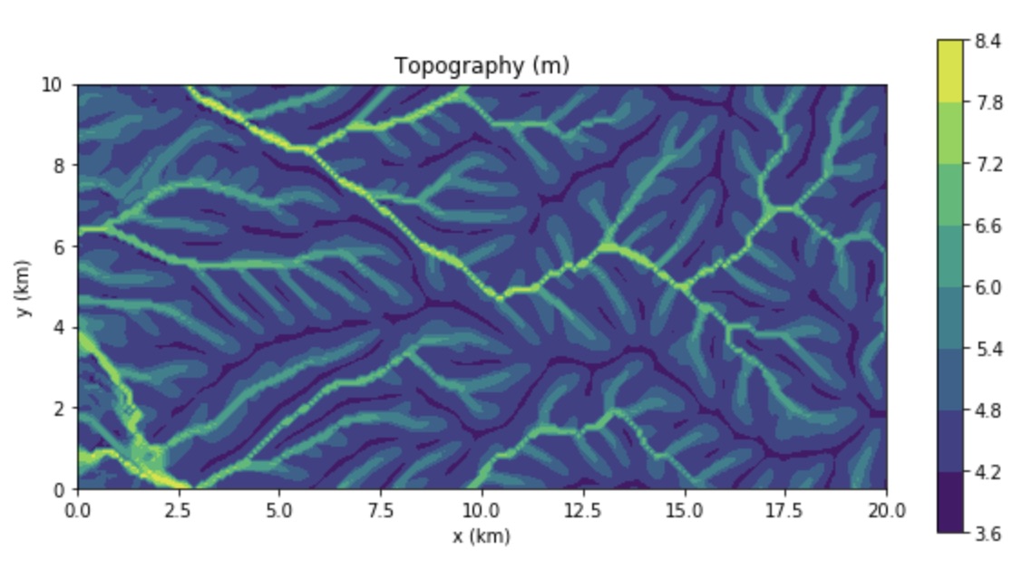
The drainage area of the last time step is also shown as a contour plot as shown in Figure Fan example.
References
-
Braun, J. and Willett, S.D., 2013. A very efficient, O(n), implicit and parallel method to solve the basic stream power law equation governing fluvial incision and landscape evolution. Geomorphology, 180-181, pp., 170-179.
-
Cordonnier, G., Bovy, B. and Braun, J., 2019. A versatile, linear complexity algorithm for flow routing in topographies with depressions. Earth Surf. Dynam., 7, pp. 549–562.
-
Yuan, X., Braun, J., Guerit, L., Rouby, D. and Cordonnier, G., 2019. A New Efficient Method to Solve the Stream Power Law Model Taking Into Account Sediment Deposition. Journal of Geohysical Research - Surface, 124 (6), pp. 1346-1365.
-
Yuan, X., Braun, J., Guerit, L., Simon, B., Bovy, B., Rouby, D., Robin, C. and Jiao, R., 2019. Linking continental deposition to marine sediment transport and deposition: a new implicit and o(n) method for inverse analysis. Earth and Planetary Science Letters, 524, 115728.
Release notes
Version 2.9.0 (Unreleased)
Changes
Bug fixes
Version 2.8.4 (29 September 2023)
Changes
-
Update source and online documentation of silt fraction #54
Bug fixes
-
Fixed compilation issues #56
Version 2.8.3 (2 December 2022)
Changes
-
Added user parametrable relative and absolute convergence parameters #51
-
VTK: set output files endianness using flags instead of within the code #47
-
VTK: added Filled Stratigraphic file for easier viewing and producing wells #41
Bug fixes
-
Fixed various warnings and errors #47
-
Added a couple of missing type declaration statements #43
-
Fixed bug in estimating erosional flux #39
Version 2.8.2 (19 May 2020)
Changes
-
Improved the documentation on installing Python bindings #37
Bug fixes
-
Made internal changes for more flexibility downstream #25
-
Refactored boundary conditions #33
-
Fixed boundary conditions in flexure #34
-
Explicit deallocation of arrays in StreamPowerLaw routines #35
-
Fixed some build issues with recent NumPy versions #37
-
Simplified CMake script for building the Python extension #37
-
Moved lake depth computation in flow routing subroutines #38
Version 2.8.1 (13 October 2019)
Bug fixes
-
Fixed regression with boundary conditions and StreamPowerLaw #29
Version 2.8.0 (18 September 2019)
Changes
-
Refactor stream power law implementation (decouple from flow routing) #23
-
Rename Union internal subroutine (could cause name conflicts when building the library with f2py) #22
New features
-
New routines for computing curvature and slope #15
-
New component for marine sediment transport and deposition #20
Bug fixes
-
Fixed VTK files export on Windows #7
-
Improved efficiency of stream power law erosion and flexure #8
-
Fixed bug in lake filling algorithm #12
-
Fixed bug in ADI implementation of diffusion #17
-
Fixed bug in Strati subroutine #18
Version 2.7.0 (30 January 2019)
-
First release in VCS.